Rank predictions at a specific time point

Usage

# S3 method for class 'mb.predict'
rank(
  x,
  time = max(x$summary[[1]]$time),
  lower_better = FALSE,
  treats = names(x$summary),
  ...
)

Arguments

x: an object of class("mb.predict") that contains predictions from an MBNMA model
time: a number indicating the time point at which predictions should be ranked. It must be one of the time points for which predictions in x are available.
lower_better: Indicates whether negative responses are better (lower_better=TRUE) or positive responses are better (lower_better=FALSE)
treats: A character vector of treatment/class names for which responses have been predicted in x As default, rankings will be calculated for all treatments/classes in x.
...: Arguments to be passed to methods

Value

Returns an object of class("mb.rank") containing ranked predictions

Examples

# \donttest{
# Create an mb.network object from a dataset
network <- mb.network(osteopain)
#> Reference treatment is `Pl_0`
#> Studies reporting change from baseline automatically identified from the data

# Run an MBNMA model with an Emax time-course
emax <- mb.run(network,
  fun=temax(pool.emax="rel", method.emax="common",
    pool.et50="abs", method.et50="common"))
#> 'et50' parameters must take positive values.
#>  Default half-normal prior restricts posterior to positive values.
#> Compiling model graph
#>    Resolving undeclared variables
#>    Allocating nodes
#> Graph information:
#>    Observed stochastic nodes: 417
#>    Unobserved stochastic nodes: 89
#>    Total graph size: 7703
#> 
#> Initializing model
#> 

# Predict responses using a stochastic baseline (E0) and a distribution for the
#network reference treatment
preds <- predict(emax, E0=7,
  ref.resp=list(emax=~rnorm(n, -0.5, 0.05)))
#> Priors required for: mu.1
#> Success: Elements in prior match consistency time-course treatment effect parameters

# Rank predictions at latest predicted time-point
rank(preds, lower_better=TRUE)
#> 
#> ========================================
#> Treatment rankings
#> ======================================== 
#> 
#> Predictions at time = 24 ranking
#> 
#> |Treatment |  Mean| Median| 2.5%| 97.5%|
#> |:---------|-----:|------:|----:|-----:|
#> |Pl_0      | 27.61|     28|   26| 28.00|
#> |Ce_100    | 21.88|     22|   18| 23.00|
#> |Ce_200    | 13.78|     14|   11| 17.00|
#> |Ce_400    | 10.92|     11|    7| 17.00|
#> |Du_90     | 20.99|     22|   11| 25.00|
#> |Et_10     | 26.37|     26|   24| 28.00|
#> |Et_30     |  6.89|      7|    4|  9.00|
#> |Et_5      | 26.27|     26|   24| 28.00|
#> |Et_60     |  2.50|      2|    2|  3.00|
#> |Et_90     |  2.52|      3|    2|  3.00|
#> |Lu_100    | 16.21|     16|   12| 20.00|
#> |Lu_200    | 16.77|     17|   12| 21.00|
#> |Lu_400    | 10.06|     10|    7| 14.00|
#> |Lu_NA     | 12.39|     12|    7| 21.00|
#> |Na_1000   |  5.09|      5|    4|  7.00|
#> |Na_1500   |  7.05|      7|    5| 10.00|
#> |Na_250    | 28.98|     29|   29| 29.00|
#> |Na_750    | 14.54|     14|   10| 20.00|
#> |Ox_44     |  7.06|      6|    4| 18.03|
#> |Ro_12     | 15.95|     16|   10| 22.00|
#> |Ro_125    |  1.00|      1|    1|  1.00|
#> |Ro_25     |  5.57|      5|    4|  9.00|
#> |Tr_100    | 25.49|     25|   24| 27.00|
#> |Tr_200    | 24.16|     24|   23| 26.00|
#> |Tr_300    | 19.77|     20|   15| 23.00|
#> |Tr_400    | 17.60|     18|   11| 22.00|
#> |Va_10     | 18.70|     19|   11| 23.00|
#> |Va_20     | 11.42|     11|    7| 19.00|
#> |Va_5      | 17.46|     18|   10| 23.00|
#> 
#> 


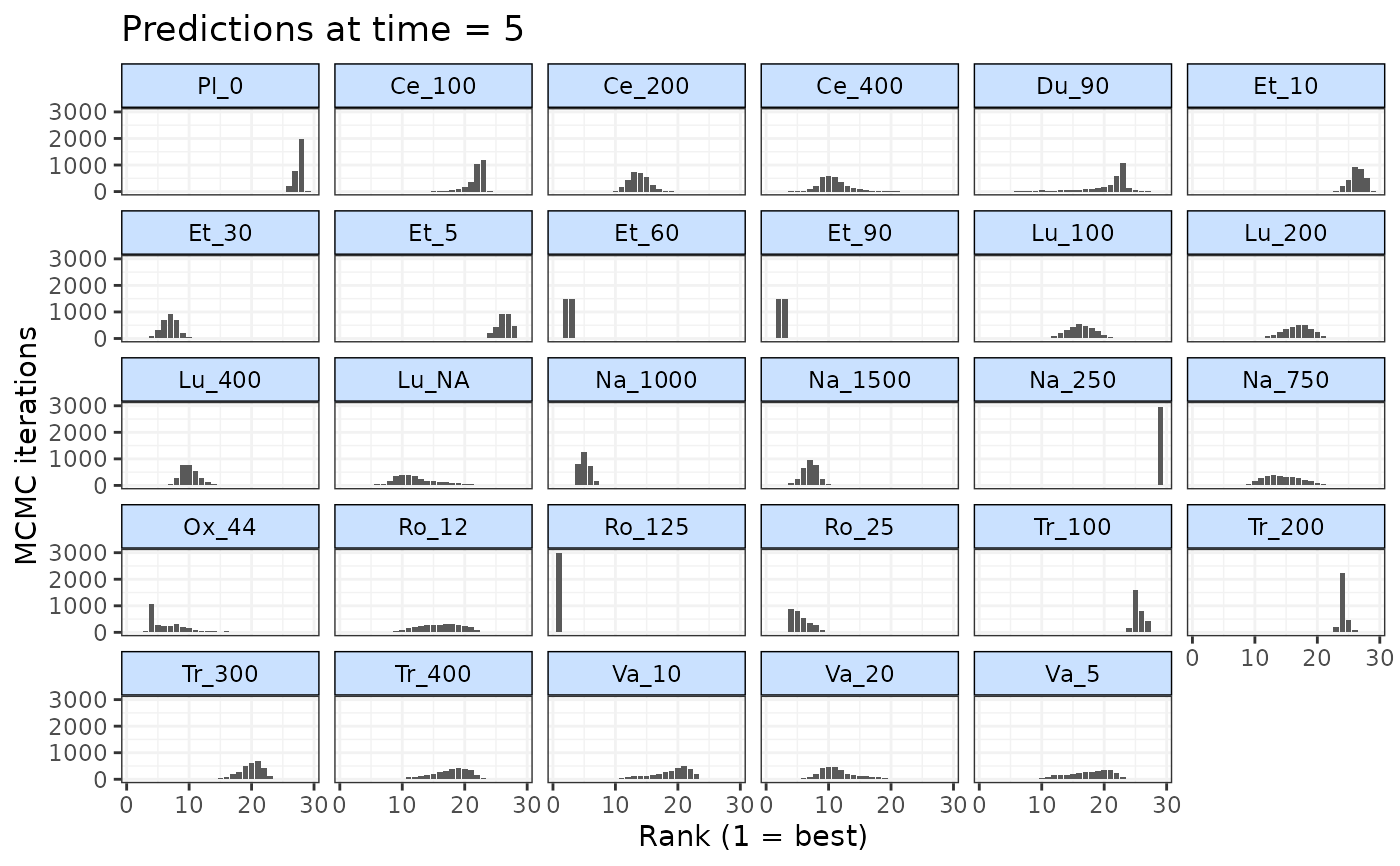
#### Rank predictions at 5 weeks follow-up ####

# First ensure responses are predicted at 5 weeks
preds <- predict(emax, E0=7,
  ref.resp=list(emax=~rnorm(n, -0.5, 0.05)),
  times=c(0,5,10))
#> Priors required for: mu.1
#> Success: Elements in prior match consistency time-course treatment effect parameters

# Rank predictions at 5 weeks follow-up
ranks <- rank(preds, lower_better=TRUE, time=5)

# Plot ranks
plot(ranks)


# }