Run MBNMA time-course models — mb.run • MBNMAtime

Fits a Bayesian time-course model for model-based network meta-analysis (MBNMA) that can account for repeated measures over time within studies by applying a desired time-course function. Follows the methods of pedder2019;textualMBNMAtime.

Usage

mb.run(
  network,
  fun = tpoly(degree = 1),
  positive.scale = FALSE,
  intercept = NULL,
  link = "identity",
  sdscale = FALSE,
  parameters.to.save = NULL,
  rho = 0,
  covar = "varadj",
  corparam = FALSE,
  class.effect = list(),
  UME = FALSE,
  parallel = FALSE,
  priors = NULL,
  n.iter = 20000,
  n.chains = 3,
  n.burnin = floor(n.iter/2),
  n.thin = max(1, floor((n.iter - n.burnin)/1000)),
  pD = TRUE,
  model.file = NULL,
  jagsdata = NULL,
  ...
)

Arguments

network

An object of class "mb.network".

fun

An object of class "timefun" generated (see Details) using any of tloglin(), tpoly(), titp(), temax(), tfpoly(), tspline() or tuser()

positive.scale

A boolean object that indicates whether all continuous mean responses (y) are positive and therefore whether the baseline response should be given a prior that constrains it to be positive (e.g. for scales that cannot be <0).

intercept

A boolean object that indicates whether an intercept (written as alpha in the model) is to be included. If left as NULL (the default), an intercept will be included only for studies reporting absolute means, and will be excluded for studies reporting change from baseline (as indicated in network$cfb).

link

Can take either "identity" (the default), "log" (for modelling Ratios of Means friedrich2011MBNMAtime) or "smd" (for modelling Standardised Mean Differences - although this also corresponds to an identity link function).

sdscale

Logical object to indicate whether to write a model that specifies a reference SD for standardising when modelling using Standardised Mean Differences. Specifying sdscale=TRUE will therefore only modify the model if link function is set to SMD (link="smd").

parameters.to.save

A character vector containing names of parameters to monitor in JAGS

rho

The correlation coefficient when modelling within-study correlation between time points. The default is a string representing a prior distribution in JAGS, indicating that it be estimated from the data (e.g. rho="dunif(0,1)"). rho also be assigned a numeric value (e.g. rho=0.7), which fixes rho in the model to this value (e.g. for use in a deterministic sensitivity analysis). If set to rho=0 (the default) then this implies modelling no correlation between time points.

covar

A character specifying the covariance structure to use for modelling within-study correlation between time-points. This can be done by specifying one of the following:

"varadj" - a univariate likelihood with a variance adjustment to assume a constant correlation between subsequent time points jansen2015MBNMAtime. This is the default.
"CS" - a multivariate normal likelihood with a compound symmetry structure
"AR1" - a multivariate normal likelihood with an autoregressive AR1 structure

corparam

A boolean object that indicates whether correlation should be modeled between relative effect time-course parameters. Default is FALSE and this is automatically set to FALSE if class effects are modeled. Setting it to TRUE models correlation between time-course parameters. This can help identify parameters that are estimated poorly for some treatments by allowing sharing of information between parameters for different treatments in the network, but may also cause some shrinkage.

class.effect

A list of named strings that determines which time-course parameters to model with a class effect and what that effect should be ("common" or "random"). For example: list(emax="common", et50="random").

UME

Can take either TRUE or FALSE (for an unrelated mean effects model on all or no time-course parameters respectively) or can be a vector of parameter name strings to model as UME. For example: c("beta.1", "beta.2").

parallel

A boolean value that indicates whether JAGS should be run in parallel (TRUE) or not (FALSE). If TRUE then the number of cores to use is automatically calculated. Functions that involve updating the model (e.g. devplot(), fitplot()) cannot be used with models implemented in parallel.

priors

A named list of parameter values (without indices) and replacement prior distribution values given as strings using distributions as specified in JAGS syntax (see jagsmanual;textualMBNMAtime).

n.iter

number of total iterations per chain (including burn in; default: 20000)

n.chains

number of Markov chains (default: 3)

n.burnin

length of burn in, i.e. number of iterations to discard at the beginning. Default is n.iter/2``, that is, discarding the first half of the simulations. If n.burnin` is 0, jags() will run 100 iterations for adaption.

n.thin

thinning rate. Must be a positive integer. Set n.thin > 1`` to save memory and computation time if n.iteris large. Default ismax(1, floor(n.chains * (n.iter-n.burnin) / 1000))“ which will only thin if there are at least 2000 simulations.

pD

logical; if TRUE (the default) then adds the computation of pD, using the method of plummer2008MBNMAtime. If FALSE then uses the approximation of pD=var(deviance) / 2 (often referred to as pV).

model.file

The file path to a JAGS model (.jags file) that can be used to overwrite the JAGS model that is automatically written based on the specified options in MBNMAtime. Useful for adding further model flexibility.

jagsdata

A named list of the data objects to be used in the JAGS model. Only required if users are defining their own JAGS model using model.file. Format should match that of standard models fitted in MBNMAtime (see mbnma$model.arg$jagsdata)

...

Arguments to be sent to R2jags.

Value

An object of S3 class c("mbnma", "rjags")`` containing parameter results from the model. Can be summarized by print()and can check traceplots usingR2jags::traceplot()or various functions from the packagemcmcplots`.#'

If there are errors in the JAGS model code then the object will be a list consisting of two elements - an error message from JAGS that can help with debugging and model.arg, a list of arguments provided to mb.run() which includes jagscode, the JAGS code for the model that can help users identify the source of the error.

Time-course parameters

Nodes that are automatically monitored (if present in the model) have the same name as in the time-course function for named time-course parameters (e.g. emax). However, for named only as beta.1, beta.2, beta.3 or beta.4 parameters may have an alternative interpretation.

Details of the interpretation and model specification of different parameters can be shown by using the summary() method on an "mbnma" object generated by mb.run().

Parameters modelled using relative effects

If pooling is relative (e.g. pool.1="rel") for a given parameter then the named parameter (e.g. emax) or a numbered d parameter (e.g. d.1) corresponds to the pooled relative effect for a given treatment compared to the network reference treatment for this time-course parameter.
sd. followed by a named (e.g. emax, beta.1) is the between-study SD (heterogeneity) for relative effects, reported if pooling for a time-course parameter is relative (e.g. pool.1="rel") and the method for synthesis is random (e.g. method.1="random).
If class effects are modelled, parameters for classes are represented by the upper case name of the time-course parameter they correspond to. For example if class.effect=list(emax="random"), relative class effects will be represented by EMAX. The SD of the class effect (e.g. sd.EMAX, sd.BETA.1) is the SD of treatments within a class for the time-course parameter they correspond to.

Parameters modelled using absolute effects

If pooling is absolute (e.g. pool.1="abs") for a given parameter then the named parameter (e.g. emax) or a numbered beta parameter (e.g. beta.1) corresponds to the estimated absolute effect for this time-course parameter.
For an absolute time-course parameter if the corresponding method is common (e.g. method.1="common") the parameter corresponds to a single common parameter estimated across all studies and treatments. If the corresponding method is random (e.g. method.1="random") then parameter is a mean effect around which the study-level absolute effects vary with SD corresponding to sd. followed by the named parameter (e.g. sd.emax, sd.beta.1) .

Other model parameters

rho The correlation coefficient for correlation between time-points. Its interpretation will differ depending on the covariance structure specified in covar
totresdev The residual deviance of the model
deviance The deviance of the model

Time-course function

Several general time-course functions with up to 4 time-course parameters are provided, but a user-defined time-course relationship can instead be used. Details can be found in the respective help files for each function.

Available time-course functions are:

Log-linear: tloglin()
Polynomial: tpoly()
Integrated Two-Component Prediction (ITP): titp()
Emax: temax()
Fractional polynomial: tfpoly()
Splines (various spline types can be used): tspline()
User-defined: tuser()

Correlation between observations

When modelling correlation between observations using rho, values for rho must imply a positive semidefinite covariance matrix.

Advanced options

model.file and jagsdata can be used to run an edited JAGS model and dataset. This allows users considerably more modelling flexibility than is possible using the basic MBNMAtime syntax, though requires strong understanding of JAGS and the MBNMA modelling framework. Treatment-specific priors, meta-regression and bias-adjustment are all possible in this way, and it allows users to make use of the subsequent functions in MBNMAtime (plotting, prediction, ranking) whilst fitting these more complex models.

References

Examples

# \donttest{
# Create mb.network object
network <- mb.network(osteopain)
#> Reference treatment is `Pl_0`
#> Studies reporting change from baseline automatically identified from the data

# Fit a linear time-course MBNMA with:
# random relative treatment effects on the slope
mb.run(network, fun=tpoly(degree=1, pool.1="rel", method.1="random"))
#> Compiling model graph
#>    Resolving undeclared variables
#>    Allocating nodes
#> Graph information:
#>    Observed stochastic nodes: 417
#>    Unobserved stochastic nodes: 163
#>    Total graph size: 7701
#> 
#> Initializing model
#> 
#> Inference for Bugs model at "/tmp/RtmpPWTcs6/file1eda782fc3e5", fit using jags,
#>  3 chains, each with 20000 iterations (first 10000 discarded), n.thin = 10
#>  n.sims = 3000 iterations saved. Running time = 7.582 secs
#>            mu.vect sd.vect     2.5%      25%      50%      75%    97.5%  Rhat
#> d.1[1]       0.000   0.000    0.000    0.000    0.000    0.000    0.000 1.000
#> d.1[2]      -0.064   0.046   -0.155   -0.094   -0.063   -0.035    0.024 1.002
#> d.1[3]      -0.094   0.018   -0.129   -0.106   -0.094   -0.082   -0.058 1.001
#> d.1[4]      -0.094   0.044   -0.180   -0.123   -0.093   -0.065   -0.009 1.001
#> d.1[5]      -0.043   0.053   -0.147   -0.079   -0.043   -0.008    0.062 1.002
#> d.1[6]       0.002   0.070   -0.138   -0.045    0.002    0.050    0.142 1.001
#> d.1[7]      -0.148   0.035   -0.218   -0.171   -0.148   -0.125   -0.083 1.001
#> d.1[8]      -0.028   0.069   -0.169   -0.072   -0.029    0.016    0.106 1.002
#> d.1[9]      -0.290   0.049   -0.389   -0.322   -0.289   -0.257   -0.196 1.001
#> d.1[10]     -0.306   0.070   -0.445   -0.353   -0.305   -0.258   -0.169 1.001
#> d.1[11]     -0.076   0.038   -0.152   -0.102   -0.075   -0.051   -0.001 1.001
#> d.1[12]     -0.069   0.037   -0.142   -0.093   -0.069   -0.044    0.004 1.002
#> d.1[13]     -0.084   0.046   -0.173   -0.116   -0.083   -0.052    0.007 1.001
#> d.1[14]     -0.082   0.063   -0.208   -0.123   -0.083   -0.041    0.043 1.001
#> d.1[15]     -0.128   0.025   -0.178   -0.145   -0.128   -0.111   -0.078 1.001
#> d.1[16]     -0.135   0.039   -0.211   -0.162   -0.135   -0.109   -0.058 1.001
#> d.1[17]      0.112   0.066   -0.024    0.069    0.113    0.155    0.244 1.002
#> d.1[18]     -0.128   0.049   -0.221   -0.159   -0.128   -0.097   -0.031 1.001
#> d.1[19]     -0.123   0.077   -0.277   -0.173   -0.124   -0.073    0.034 1.001
#> d.1[20]     -0.115   0.048   -0.213   -0.145   -0.114   -0.083   -0.021 1.001
#> d.1[21]     -0.426   0.079   -0.580   -0.478   -0.429   -0.373   -0.273 1.001
#> d.1[22]     -0.171   0.042   -0.256   -0.199   -0.170   -0.144   -0.088 1.001
#> d.1[23]     -0.031   0.041   -0.113   -0.058   -0.031   -0.004    0.049 1.001
#> d.1[24]     -0.040   0.042   -0.120   -0.068   -0.041   -0.012    0.042 1.002
#> d.1[25]     -0.067   0.042   -0.150   -0.093   -0.066   -0.039    0.015 1.001
#> d.1[26]     -0.085   0.063   -0.209   -0.125   -0.085   -0.044    0.037 1.001
#> d.1[27]     -0.067   0.066   -0.196   -0.112   -0.067   -0.024    0.062 1.001
#> d.1[28]     -0.094   0.065   -0.220   -0.138   -0.094   -0.049    0.035 1.001
#> d.1[29]     -0.078   0.066   -0.210   -0.123   -0.078   -0.034    0.054 1.001
#> rho          0.000   0.000    0.000    0.000    0.000    0.000    0.000 1.000
#> sd.beta.1    0.073   0.009    0.056    0.066    0.072    0.079    0.094 1.001
#> totresdev 9298.979  16.866 9267.942 9287.281 9298.448 9309.983 9333.912 1.001
#> deviance  8418.940  16.866 8387.903 8407.242 8418.408 8429.944 8453.873 1.001
#>           n.eff
#> d.1[1]        1
#> d.1[2]     1600
#> d.1[3]     3000
#> d.1[4]     3000
#> d.1[5]     1600
#> d.1[6]     3000
#> d.1[7]     3000
#> d.1[8]     1200
#> d.1[9]     3000
#> d.1[10]    3000
#> d.1[11]    2000
#> d.1[12]    3000
#> d.1[13]    3000
#> d.1[14]    2300
#> d.1[15]    3000
#> d.1[16]    3000
#> d.1[17]    1900
#> d.1[18]    2500
#> d.1[19]    2500
#> d.1[20]    3000
#> d.1[21]    3000
#> d.1[22]    3000
#> d.1[23]    3000
#> d.1[24]    2400
#> d.1[25]    3000
#> d.1[26]    3000
#> d.1[27]    2100
#> d.1[28]    3000
#> d.1[29]    3000
#> rho           1
#> sd.beta.1  3000
#> totresdev  2100
#> deviance   2100
#> 
#> For each parameter, n.eff is a crude measure of effective sample size,
#> and Rhat is the potential scale reduction factor (at convergence, Rhat=1).
#> 
#> DIC info (using the rule: pV = var(deviance)/2)
#> pV = 142.2 and DIC = 8549.8
#> DIC info (using the rule: pD = Dbar-Dhat, computed via 'rjags::dic.samples')
#> pD = 131.4 and DIC = 8549.7
#> DIC is an estimate of expected predictive error (lower deviance is better).

# Fit an emax time-course MBNMA with:
# fixed relative treatment effects on emax
# a common parameter estimated independently of treatment
# a common Hill parameter estimated independently of treatment
# a prior for the Hill parameter (normal with mean 0 and precision 0.1)
# data reported as change from baseline
result <- mb.run(network, fun=temax(pool.emax="rel", method.emax="common",
                                    pool.et50="abs", method.et50="common",
                                    pool.hill="abs", method.hill="common"),
                 priors=list(hill="dunif(0.5, 2)"),
                 intercept=TRUE)
#> 'et50' parameters must take positive values.
#>  Default half-normal prior restricts posterior to positive values.
#> 'hill' parameters must take positive values.
#>  Default half-normal prior restricts posterior to positive values.
#> Compiling model graph
#>    Resolving undeclared variables
#>    Allocating nodes
#> Graph information:
#>    Observed stochastic nodes: 417
#>    Unobserved stochastic nodes: 90
#>    Total graph size: 7740
#> 
#> Initializing model
#> 


#### commented out to prevent errors from JAGS version in github actions build ####
# Fit a log-linear MBNMA with:
# random relative treatment effects on the rate
# an autoregressive AR1 covariance structure
# modelled as standardised mean differences
# copdnet <- mb.network(copd)
# result <- mb.run(copdnet, fun=tloglin(pool.rate="rel", method.rate="random"),
#                covar="AR1", rho="dunif(0,1)", link="smd")



####### Examine MCMC diagnostics (using mcmcplots package) #######

# Traceplots
# mcmcplots::traplot(result)

# Plots for assessing convergence
# mcmcplots::mcmcplot(result, c("rate", "sd.rate", "rho"))

########## Output ###########

# Print R2jags output and summary
print(result)
#> Inference for Bugs model at "/tmp/RtmpPWTcs6/file1eda455b940b", fit using jags,
#>  3 chains, each with 20000 iterations (first 10000 discarded), n.thin = 10
#>  n.sims = 3000 iterations saved. Running time = 44.971 secs
#>           mu.vect sd.vect    2.5%     25%     50%     75%   97.5%  Rhat n.eff
#> emax[1]     0.000   0.000   0.000   0.000   0.000   0.000   0.000 1.000     1
#> emax[2]    -0.643   0.106  -0.851  -0.714  -0.642  -0.571  -0.432 1.001  3000
#> emax[3]    -0.934   0.044  -1.017  -0.964  -0.935  -0.905  -0.847 1.002  1200
#> emax[4]    -1.043   0.104  -1.250  -1.111  -1.043  -0.971  -0.843 1.001  3000
#> emax[5]    -0.640   0.198  -1.031  -0.770  -0.637  -0.512  -0.248 1.001  3000
#> emax[6]    -0.112   0.141  -0.394  -0.211  -0.112  -0.016   0.162 1.001  3000
#> emax[7]    -1.231   0.070  -1.370  -1.275  -1.230  -1.184  -1.095 1.002  1100
#> emax[8]    -0.115   0.143  -0.397  -0.211  -0.115  -0.022   0.179 1.001  3000
#> emax[9]    -1.896   0.108  -2.111  -1.969  -1.895  -1.823  -1.683 1.001  3000
#> emax[10]   -1.896   0.156  -2.207  -2.000  -1.897  -1.791  -1.601 1.002  1200
#> emax[11]   -0.878   0.061  -0.998  -0.920  -0.878  -0.837  -0.760 1.001  3000
#> emax[12]   -0.861   0.063  -0.983  -0.903  -0.860  -0.818  -0.735 1.001  3000
#> emax[13]   -1.064   0.076  -1.216  -1.116  -1.063  -1.013  -0.917 1.001  3000
#> emax[14]   -0.996   0.124  -1.244  -1.079  -0.994  -0.914  -0.755 1.002  1000
#> emax[15]   -1.318   0.064  -1.443  -1.362  -1.320  -1.275  -1.190 1.003  1400
#> emax[16]   -1.224   0.074  -1.369  -1.275  -1.223  -1.172  -1.080 1.004   520
#> emax[17]    0.359   0.138   0.088   0.266   0.355   0.452   0.633 1.001  3000
#> emax[18]   -0.927   0.088  -1.097  -0.986  -0.927  -0.866  -0.760 1.004   530
#> emax[19]   -1.287   0.237  -1.763  -1.443  -1.286  -1.125  -0.825 1.005   470
#> emax[20]   -0.882   0.101  -1.084  -0.949  -0.882  -0.814  -0.686 1.001  2800
#> emax[21]   -2.641   0.205  -3.036  -2.779  -2.638  -2.503  -2.248 1.002  1600
#> emax[22]   -1.311   0.114  -1.541  -1.393  -1.313  -1.231  -1.091 1.002  1300
#> emax[23]   -0.213   0.069  -0.349  -0.261  -0.213  -0.167  -0.079 1.001  3000
#> emax[24]   -0.332   0.070  -0.473  -0.378  -0.329  -0.285  -0.199 1.002  1400
#> emax[25]   -0.766   0.071  -0.905  -0.813  -0.767  -0.717  -0.629 1.004   590
#> emax[26]   -0.830   0.096  -1.020  -0.894  -0.831  -0.764  -0.647 1.002  1900
#> emax[27]   -0.787   0.120  -1.024  -0.868  -0.785  -0.707  -0.549 1.002  1600
#> emax[28]   -1.025   0.123  -1.264  -1.111  -1.022  -0.938  -0.789 1.001  3000
#> emax[29]   -0.832   0.120  -1.070  -0.912  -0.833  -0.751  -0.594 1.001  3000
#> et50        0.462   0.044   0.383   0.431   0.459   0.490   0.556 1.004   660
#> hill        0.578   0.069   0.502   0.524   0.558   0.615   0.756 1.009   470
#> rho         0.000   0.000   0.000   0.000   0.000   0.000   0.000 1.000     1
#> totresdev 837.536  13.491 813.247 828.124 836.913 846.042 865.878 1.001  3000
#> deviance  -42.504  13.491 -66.793 -51.916 -43.126 -33.997 -14.161 1.001  3000
#> 
#> For each parameter, n.eff is a crude measure of effective sample size,
#> and Rhat is the potential scale reduction factor (at convergence, Rhat=1).
#> 
#> DIC info (using the rule: pV = var(deviance)/2)
#> pV = 91.0 and DIC = 46.6
#> DIC info (using the rule: pD = Dbar-Dhat, computed via 'rjags::dic.samples')
#> pD = 89.8 and DIC = 47.1
#> DIC is an estimate of expected predictive error (lower deviance is better).
summary(result)
#> ========================================
#> Time-course MBNMA
#> ========================================
#> 
#> Time-course function: emax
#> Data modelled with intercept
#> 
#> emax parameter
#> Pooling: relative effects
#> Method: common treatment effects
#> 
#> |Treatment |Parameter |  Median|    2.5%|   97.5%|
#> |:---------|:---------|-------:|-------:|-------:|
#> |Pl_0      |emax[1]   |  0.0000|  0.0000|  0.0000|
#> |Ce_100    |emax[2]   | -0.6423| -0.8510| -0.4317|
#> |Ce_200    |emax[3]   | -0.9351| -1.0171| -0.8471|
#> |Ce_400    |emax[4]   | -1.0429| -1.2504| -0.8425|
#> |Du_90     |emax[5]   | -0.6375| -1.0310| -0.2484|
#> |Et_10     |emax[6]   | -0.1124| -0.3940|  0.1615|
#> |Et_30     |emax[7]   | -1.2301| -1.3700| -1.0952|
#> |Et_5      |emax[8]   | -0.1153| -0.3968|  0.1785|
#> |Et_60     |emax[9]   | -1.8947| -2.1109| -1.6828|
#> |Et_90     |emax[10]  | -1.8967| -2.2075| -1.6006|
#> |Lu_100    |emax[11]  | -0.8781| -0.9982| -0.7599|
#> |Lu_200    |emax[12]  | -0.8600| -0.9828| -0.7351|
#> |Lu_400    |emax[13]  | -1.0630| -1.2162| -0.9168|
#> |Lu_NA     |emax[14]  | -0.9941| -1.2437| -0.7549|
#> |Na_1000   |emax[15]  | -1.3197| -1.4433| -1.1901|
#> |Na_1500   |emax[16]  | -1.2232| -1.3686| -1.0799|
#> |Na_250    |emax[17]  |  0.3545|  0.0880|  0.6334|
#> |Na_750    |emax[18]  | -0.9272| -1.0971| -0.7603|
#> |Ox_44     |emax[19]  | -1.2864| -1.7631| -0.8246|
#> |Ro_12     |emax[20]  | -0.8819| -1.0838| -0.6863|
#> |Ro_125    |emax[21]  | -2.6379| -3.0358| -2.2477|
#> |Ro_25     |emax[22]  | -1.3126| -1.5407| -1.0911|
#> |Tr_100    |emax[23]  | -0.2135| -0.3493| -0.0794|
#> |Tr_200    |emax[24]  | -0.3287| -0.4733| -0.1993|
#> |Tr_300    |emax[25]  | -0.7665| -0.9052| -0.6289|
#> |Tr_400    |emax[26]  | -0.8315| -1.0199| -0.6468|
#> |Va_10     |emax[27]  | -0.7852| -1.0240| -0.5488|
#> |Va_20     |emax[28]  | -1.0217| -1.2643| -0.7894|
#> |Va_5      |emax[29]  | -0.8325| -1.0705| -0.5943|
#> 
#> 
#> et50 parameter
#> Pooling: absolute effects
#> Method: common treatment effects
#> 
#> |Treatment |Parameter | Median|   2.5%|  97.5%|
#> |:---------|:---------|------:|------:|------:|
#> |Pl_0      |et50      | 0.4593| 0.3834| 0.5561|
#> |Ce_100    |et50      | 0.4593| 0.3834| 0.5561|
#> |Ce_200    |et50      | 0.4593| 0.3834| 0.5561|
#> |Ce_400    |et50      | 0.4593| 0.3834| 0.5561|
#> |Du_90     |et50      | 0.4593| 0.3834| 0.5561|
#> |Et_10     |et50      | 0.4593| 0.3834| 0.5561|
#> |Et_30     |et50      | 0.4593| 0.3834| 0.5561|
#> |Et_5      |et50      | 0.4593| 0.3834| 0.5561|
#> |Et_60     |et50      | 0.4593| 0.3834| 0.5561|
#> |Et_90     |et50      | 0.4593| 0.3834| 0.5561|
#> |Lu_100    |et50      | 0.4593| 0.3834| 0.5561|
#> |Lu_200    |et50      | 0.4593| 0.3834| 0.5561|
#> |Lu_400    |et50      | 0.4593| 0.3834| 0.5561|
#> |Lu_NA     |et50      | 0.4593| 0.3834| 0.5561|
#> |Na_1000   |et50      | 0.4593| 0.3834| 0.5561|
#> |Na_1500   |et50      | 0.4593| 0.3834| 0.5561|
#> |Na_250    |et50      | 0.4593| 0.3834| 0.5561|
#> |Na_750    |et50      | 0.4593| 0.3834| 0.5561|
#> |Ox_44     |et50      | 0.4593| 0.3834| 0.5561|
#> |Ro_12     |et50      | 0.4593| 0.3834| 0.5561|
#> |Ro_125    |et50      | 0.4593| 0.3834| 0.5561|
#> |Ro_25     |et50      | 0.4593| 0.3834| 0.5561|
#> |Tr_100    |et50      | 0.4593| 0.3834| 0.5561|
#> |Tr_200    |et50      | 0.4593| 0.3834| 0.5561|
#> |Tr_300    |et50      | 0.4593| 0.3834| 0.5561|
#> |Tr_400    |et50      | 0.4593| 0.3834| 0.5561|
#> |Va_10     |et50      | 0.4593| 0.3834| 0.5561|
#> |Va_20     |et50      | 0.4593| 0.3834| 0.5561|
#> |Va_5      |et50      | 0.4593| 0.3834| 0.5561|
#> 
#> 
#> hill parameter
#> Pooling: absolute effects
#> Method: common treatment effects
#> 
#> |Treatment |Parameter | Median|   2.5%|  97.5%|
#> |:---------|:---------|------:|------:|------:|
#> |Pl_0      |hill      | 0.5584| 0.5023| 0.7563|
#> |Ce_100    |hill      | 0.5584| 0.5023| 0.7563|
#> |Ce_200    |hill      | 0.5584| 0.5023| 0.7563|
#> |Ce_400    |hill      | 0.5584| 0.5023| 0.7563|
#> |Du_90     |hill      | 0.5584| 0.5023| 0.7563|
#> |Et_10     |hill      | 0.5584| 0.5023| 0.7563|
#> |Et_30     |hill      | 0.5584| 0.5023| 0.7563|
#> |Et_5      |hill      | 0.5584| 0.5023| 0.7563|
#> |Et_60     |hill      | 0.5584| 0.5023| 0.7563|
#> |Et_90     |hill      | 0.5584| 0.5023| 0.7563|
#> |Lu_100    |hill      | 0.5584| 0.5023| 0.7563|
#> |Lu_200    |hill      | 0.5584| 0.5023| 0.7563|
#> |Lu_400    |hill      | 0.5584| 0.5023| 0.7563|
#> |Lu_NA     |hill      | 0.5584| 0.5023| 0.7563|
#> |Na_1000   |hill      | 0.5584| 0.5023| 0.7563|
#> |Na_1500   |hill      | 0.5584| 0.5023| 0.7563|
#> |Na_250    |hill      | 0.5584| 0.5023| 0.7563|
#> |Na_750    |hill      | 0.5584| 0.5023| 0.7563|
#> |Ox_44     |hill      | 0.5584| 0.5023| 0.7563|
#> |Ro_12     |hill      | 0.5584| 0.5023| 0.7563|
#> |Ro_125    |hill      | 0.5584| 0.5023| 0.7563|
#> |Ro_25     |hill      | 0.5584| 0.5023| 0.7563|
#> |Tr_100    |hill      | 0.5584| 0.5023| 0.7563|
#> |Tr_200    |hill      | 0.5584| 0.5023| 0.7563|
#> |Tr_300    |hill      | 0.5584| 0.5023| 0.7563|
#> |Tr_400    |hill      | 0.5584| 0.5023| 0.7563|
#> |Va_10     |hill      | 0.5584| 0.5023| 0.7563|
#> |Va_20     |hill      | 0.5584| 0.5023| 0.7563|
#> |Va_5      |hill      | 0.5584| 0.5023| 0.7563|
#> 
#> 
#> 
#> Correlation between time points
#> Covariance structure: varadj 
#> Rho assigned a numeric value: 0
#> 
#> #### Model Fit Statistics ####
#> 
#> Effective number of parameters:
#> pD calculated using the Kullback-Leibler divergence = 90
#> Deviance = -43
#> Residual deviance = 837
#> Deviance Information Criterion (DIC) = 47 
#> 

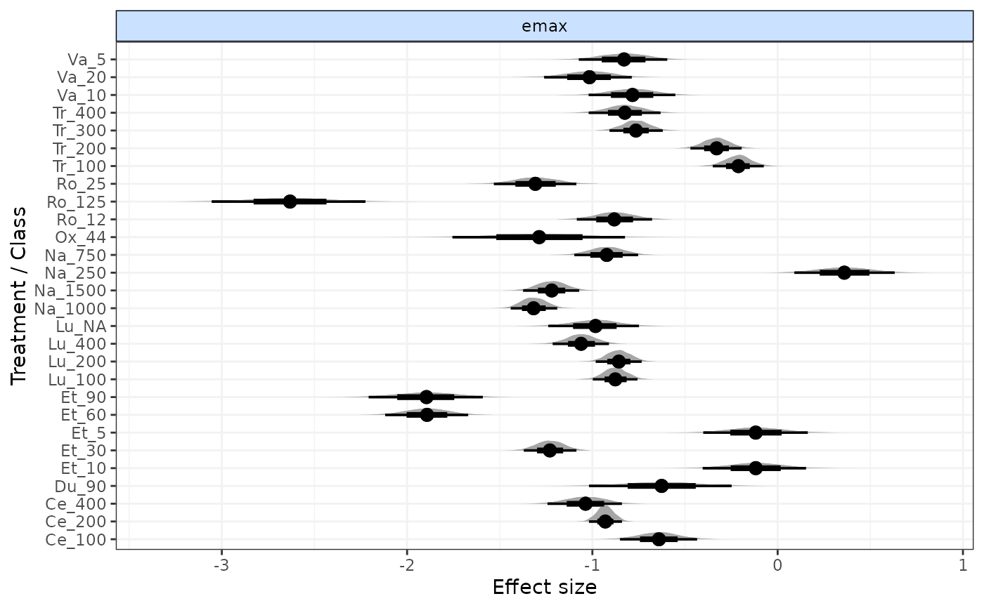
# Plot forest plot of results
plot(result)



###### Additional model arguments ######

# Use gout dataset
goutnet <- mb.network(goutSUA_CFBcomb)
#> Reference treatment is `Plac`
#> Studies reporting change from baseline automatically identified from the data

# Define a user-defined time-course relationship for use in mb.run
timecourse <- ~ exp(beta.1 * time) + (time^beta.2)

# Run model with:
# user-defined time-course function
# random relative effects on beta.1
# default common effects on beta.2
# default relative pooling on beta.1 and beta.2
# common class effect on beta.2
mb.run(goutnet, fun=tuser(fun=timecourse, method.1="random"),
       class.effect=list(beta.1="common"))
#> Compiling model graph
#>    Resolving undeclared variables
#>    Allocating nodes
#> Graph information:
#>    Observed stochastic nodes: 224
#>    Unobserved stochastic nodes: 121
#>    Total graph size: 4851
#> 
#> Initializing model
#> 
#> Inference for Bugs model at "/tmp/RtmpPWTcs6/file1eda187d45f8", fit using jags,
#>  3 chains, each with 20000 iterations (first 10000 discarded), n.thin = 10
#>  n.sims = 3000 iterations saved. Running time = 34.452 secs
#>               mu.vect sd.vect        2.5%         25%         50%         75%
#> D.1[1]          0.000   0.000       0.000       0.000       0.000       0.000
#> D.1[2]         -2.118  20.473     -45.968     -14.182      -3.444      10.255
#> D.1[3]        -16.930  24.838     -67.808     -31.971     -15.310      -5.130
#> D.1[4]          2.646  28.421     -42.129     -19.079       0.001      20.356
#> D.1[5]        -11.735  24.160     -59.798     -27.102     -10.668       4.538
#> D.1[6]        -22.912  12.563     -53.503     -29.500     -21.499     -14.146
#> D.1[7]        -25.003  18.966     -67.405     -36.798     -25.581     -13.029
#> d.1[1]          0.000   0.000       0.000       0.000       0.000       0.000
#> d.1[2]         -2.118  20.473     -45.968     -14.182      -3.444      10.255
#> d.1[3]         -2.118  20.473     -45.968     -14.182      -3.444      10.255
#> d.1[4]         -2.118  20.473     -45.968     -14.182      -3.444      10.255
#> d.1[5]         -2.118  20.473     -45.968     -14.182      -3.444      10.255
#> d.1[6]        -16.930  24.838     -67.808     -31.971     -15.310      -5.130
#> d.1[7]          2.646  28.421     -42.129     -19.079       0.001      20.356
#> d.1[8]          2.646  28.421     -42.129     -19.079       0.001      20.356
#> d.1[9]          2.646  28.421     -42.129     -19.079       0.001      20.356
#> d.1[10]         2.646  28.421     -42.129     -19.079       0.001      20.356
#> d.1[11]       -11.735  24.160     -59.798     -27.102     -10.668       4.538
#> d.1[12]       -22.912  12.563     -53.503     -29.500     -21.499     -14.146
#> d.1[13]       -22.912  12.563     -53.503     -29.500     -21.499     -14.146
#> d.1[14]       -22.912  12.563     -53.503     -29.500     -21.499     -14.146
#> d.1[15]       -22.912  12.563     -53.503     -29.500     -21.499     -14.146
#> d.1[16]       -25.003  18.966     -67.405     -36.798     -25.581     -13.029
#> d.1[17]       -25.003  18.966     -67.405     -36.798     -25.581     -13.029
#> d.1[18]       -25.003  18.966     -67.405     -36.798     -25.581     -13.029
#> d.1[19]       -25.003  18.966     -67.405     -36.798     -25.581     -13.029
#> d.2[1]          0.000   0.000       0.000       0.000       0.000       0.000
#> d.2[2]         -4.258  30.121     -64.362     -23.988      -3.908      15.377
#> d.2[3]          2.787  29.991     -55.663     -17.703       2.043      23.222
#> d.2[4]        -16.216  10.037     -42.182     -21.185     -13.726      -8.763
#> d.2[5]          3.251  30.239     -55.131     -16.629       2.790      23.528
#> d.2[6]        -15.286  28.572     -68.523     -33.332     -17.036       0.666
#> d.2[7]         -3.130  29.594     -61.992     -23.073      -2.284      16.988
#> d.2[8]         -8.295  27.617     -64.693     -26.056      -7.525       9.398
#> d.2[9]         -2.159  30.253     -62.801     -22.088      -2.312      17.542
#> d.2[10]        -5.797  27.870     -60.764     -24.387      -5.129      13.541
#> d.2[11]       -16.581  25.050     -68.613     -32.505     -16.125      -0.400
#> d.2[12]       -11.477  27.519     -68.633     -28.271     -10.667       6.432
#> d.2[13]        -7.374  28.075     -64.858     -25.710      -6.914      11.592
#> d.2[14]       -15.880  22.321     -64.696     -29.541     -14.189      -1.010
#> d.2[15]       -16.294  24.557     -67.466     -31.895     -15.595       0.514
#> d.2[16]         4.312  30.092     -54.318     -15.397       3.837      23.443
#> d.2[17]       -16.430  25.935     -68.444     -31.864     -16.255      -1.843
#> d.2[18]       -15.111  23.712     -63.893     -29.706     -15.057      -0.880
#> d.2[19]       -16.574  26.640     -69.535     -33.124     -16.911      -0.236
#> rho             0.000   0.000       0.000       0.000       0.000       0.000
#> sd.beta.1       3.162   2.226       0.167       1.377       2.760       4.569
#> totresdev 2013067.918   7.929 2013056.566 2013062.633 2013065.271 2013071.465
#> deviance  2012373.729   7.929 2012362.377 2012368.445 2012371.082 2012377.277
#>                 97.5%  Rhat n.eff
#> D.1[1]          0.000 1.000     1
#> D.1[2]         37.993 1.094    26
#> D.1[3]         40.861 1.327    11
#> D.1[4]         67.607 1.121    39
#> D.1[5]         35.313 1.056    44
#> D.1[6]         -3.048 1.094    51
#> D.1[7]         12.685 1.054    49
#> d.1[1]          0.000 1.000     1
#> d.1[2]         37.993 1.094    26
#> d.1[3]         37.993 1.094    26
#> d.1[4]         37.993 1.094    26
#> d.1[5]         37.993 1.094    26
#> d.1[6]         40.861 1.327    11
#> d.1[7]         67.607 1.121    39
#> d.1[8]         67.607 1.121    39
#> d.1[9]         67.607 1.121    39
#> d.1[10]        67.607 1.121    39
#> d.1[11]        35.313 1.056    44
#> d.1[12]        -3.048 1.094    51
#> d.1[13]        -3.048 1.094    51
#> d.1[14]        -3.048 1.094    51
#> d.1[15]        -3.048 1.094    51
#> d.1[16]        12.685 1.054    49
#> d.1[17]        12.685 1.054    49
#> d.1[18]        12.685 1.054    49
#> d.1[19]        12.685 1.054    49
#> d.2[1]          0.000 1.000     1
#> d.2[2]         53.906 1.002  1900
#> d.2[3]         60.605 1.001  3000
#> d.2[4]         -4.412 1.001  2100
#> d.2[5]         63.861 1.001  3000
#> d.2[6]         46.050 1.122    22
#> d.2[7]         52.753 1.001  3000
#> d.2[8]         44.331 1.002  1600
#> d.2[9]         58.187 1.001  3000
#> d.2[10]        47.087 1.002  1600
#> d.2[11]        31.086 1.003   690
#> d.2[12]        40.577 1.001  3000
#> d.2[13]        45.125 1.006   370
#> d.2[14]        25.469 1.001  3000
#> d.2[15]        29.584 1.001  2300
#> d.2[16]        65.261 1.001  3000
#> d.2[17]        37.224 1.126    22
#> d.2[18]        32.415 1.138    20
#> d.2[19]        37.934 1.162    17
#> rho             0.000 1.000     1
#> sd.beta.1       8.259 1.060    73
#> totresdev 2013085.220 1.000     1
#> deviance  2012391.032 1.000     1
#> 
#> For each parameter, n.eff is a crude measure of effective sample size,
#> and Rhat is the potential scale reduction factor (at convergence, Rhat=1).
#> 
#> DIC info (using the rule: pV = var(deviance)/2)
#> pV = 28.8 and DIC = 2012379.7
#> DIC info (using the rule: pD = Dbar-Dhat, computed via 'rjags::dic.samples')
#> pD = 8.6 and DIC = 2012382.9
#> DIC is an estimate of expected predictive error (lower deviance is better).

# Fit a log-linear MBNMA
# with variance adjustment for correlation between time-points
result <- mb.run(network, fun=tloglin(),
                 rho="dunif(0,1)", covar="varadj")
#> Compiling model graph
#>    Resolving undeclared variables
#>    Allocating nodes
#> Graph information:
#>    Observed stochastic nodes: 417
#>    Unobserved stochastic nodes: 89
#>    Total graph size: 7303
#> 
#> Initializing model
#> 
# }