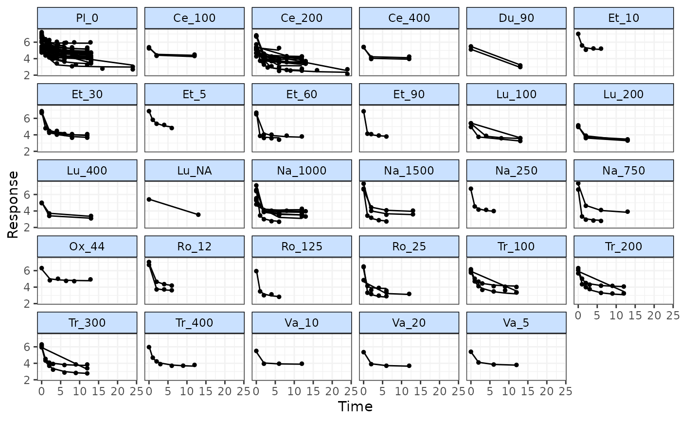
Plot fitted values from MBNMA model

Usage

fitplot(
  mbnma,
  treat.labs = NULL,
  disp.obs = TRUE,
  n.iter = round(mbnma$BUGSoutput$n.iter/4),
  n.thin = mbnma$BUGSoutput$n.thin,
  ...
)

Arguments

mbnma: An S3 object of class "mbnma" generated by running a time-course MBNMA model
treat.labs: A character vector of treatment labels with which to name graph panels. Can use mb.network()[["treatments"]] with original dataset if in doubt.
disp.obs: A boolean object to indicate whether raw data responses should be plotted as points on the graph
n.iter: number of total iterations per chain (including burn in; default: 2000)
n.thin: thinning rate. Must be a positive integer. Set n.thin > 1 to save memory and computation time if n.iter is large. Default is max(1, floor(n.chains * (n.iter-n.burnin) / 1000)) which will only thin if there are at least 2000 simulations.
...: Arguments to be sent to ggplot2::ggplot()

Value

Generates a plot of fitted values from the MBNMA model and returns a list containing the plot (as an object of class c("gg", "ggplot")), and a data.frame of posterior mean fitted values for each observation.

Details

Fitted values should only be plotted for models that have converged successfully. If fitted values (theta) have not been monitored in mbnma$parameters.to.save then additional iterations will have to be run to get results for these.

Examples

# \donttest{
# Make network
painnet <- mb.network(osteopain)
#> Reference treatment is `Pl_0`
#> Studies reporting change from baseline automatically identified from the data

# Run MBNMA
mbnma <- mb.run(painnet,
  fun=temax(pool.emax="rel", method.emax="common",
    pool.et50="abs", method.et50="random"))
#> 'et50' parameters must take positive values.
#>  Default half-normal prior restricts posterior to positive values.
#> Compiling model graph
#>    Resolving undeclared variables
#>    Allocating nodes
#> Graph information:
#>    Observed stochastic nodes: 417
#>    Unobserved stochastic nodes: 194
#>    Total graph size: 8210
#> 
#> Initializing model
#> 

# Plot fitted values from the model
# Monitor fitted values for 500 additional iterations
fitplot(mbnma, n.iter=500)
#> `theta` not monitored in mbnma$parameters.to.save.
#> additional iterations will be run in order to obtain results

# }