Calculating model predictions

Prediction

After performing an MBNMA, predictions can be calculated from the parameter estimates using predict() on an "mbnma" object. A number of important parameters need to be identified to make robust predictions. However, default values can be used that set values of zero for the reference treatment baseline and time-course parameters which indicates that mean differences / relative treatment effects should be estimated. For further information the help file can be accessed using ?predict.mbnma.

E0 (time=0)

One key parameter is E0, which defines what value(s) to use for the predicted mean at time = 0. A single numeric value can be given for E0 to indicate a deterministic value, or a function representing a random number generator (RNG) distribution in R (stochastic) (e.g. E0 = ~rnorm(n, 7, 0.2). These values can be identified for the population of interest from external data (e.g. observational/registry).

Baseline (reference treatment) time-course

The more challenging parameter(s) to identify are those for the network reference treatment time-course, supplied to predict() in the ref.resp argument. For estimating mean differences / relative treatment effects over time this does not need to be specified since typically in an MBNMA, relative effects are estimated and the network reference effect is modeled as a nuisance parameter.

However, for predicting mean responses over time we need to provide an input for the network reference treatment effect for all time-course parameters modeled using pool="rel" so that we can apply the relative effects estimated in our model to it. There are two options for providing these values.

The first approach is to give values for each time-course parameter modeled using relative effects to ref.resp. This is given as a list, with a separate named element for each time-course parameter. Each element can take either a single numeric value (deterministic), or a function representing a random number generator distribution in R (stochastic).

# Run an Emax time-course MBNMA using the osteoarthritis dataset
mbnma <- mb.run(network.pain,
                fun=temax(pool.emax="rel", method.emax="common",
                          pool.et50="abs", method.et50="common"),
                rho="dunif(0,1)", covar="varadj")

# Specify placebo time-course parameters
ref.params <- list(emax=-2)

# Predict responses for a selection of treatments using a stochastic E0 and
# placebo parameters defined in ref.params to estimate the network reference treatment effect
pred <- predict(mbnma, treats=c("Pl_0", "Ce_200", "Du_90", "Et_60", 
                                        "Lu_400", "Na_1000", "Ox_44", "Ro_25",
                                        "Tr_300", "Va_20"),
                        E0=~rnorm(n, 8, 0.5), ref.resp=ref.params)

print(pred)

The second is to assign ref.resp a data frame composed of single-arm studies of the network reference treatment. A separate synthesis model for the reference treatment effect will then be run, and the values from this used as the prediction reference treatment effect. This dataset could be a series of observational studies measured at multiple follow-up times that closely match the population of interest for the prediction. Alternatively it could be a subset of data from the original RCT dataset used for the MBNMA model (though this may be less generalisable to the population of interest).

# Generate a dataset of network reference treatment responses over time
placebo.df <- network.pain$data.ab[network.pain$data.ab$treatment==1,]

# Predict responses for a selection of treatments using a deterministic E0 and 
#placebo.df to model the network reference treatment effect
pred <- predict(mbnma, treats=c("Pl_0", "Ce_200", "Du_90", "Et_60", 
                                        "Lu_400", "Na_1000", "Ox_44", "Ro_25",
                                        "Tr_300", "Va_20"),
                        E0=10, ref.resp=placebo.df)

print(pred)

It is also possible specify the time points for which to make predictions (times), given as a vector of positive numbers. If left as the default then the maximum follow-up in the dataset will be used as the upper limit for the range of predicted time-points.

Exploring predictions

An object of class "mb.predict" is returned, which is a list of summary tables and MCMC prediction matrices for each treatment, in addition to the original mbnma object. The summary() method can be used to print mean posterior predictions at each time point for each treatment.

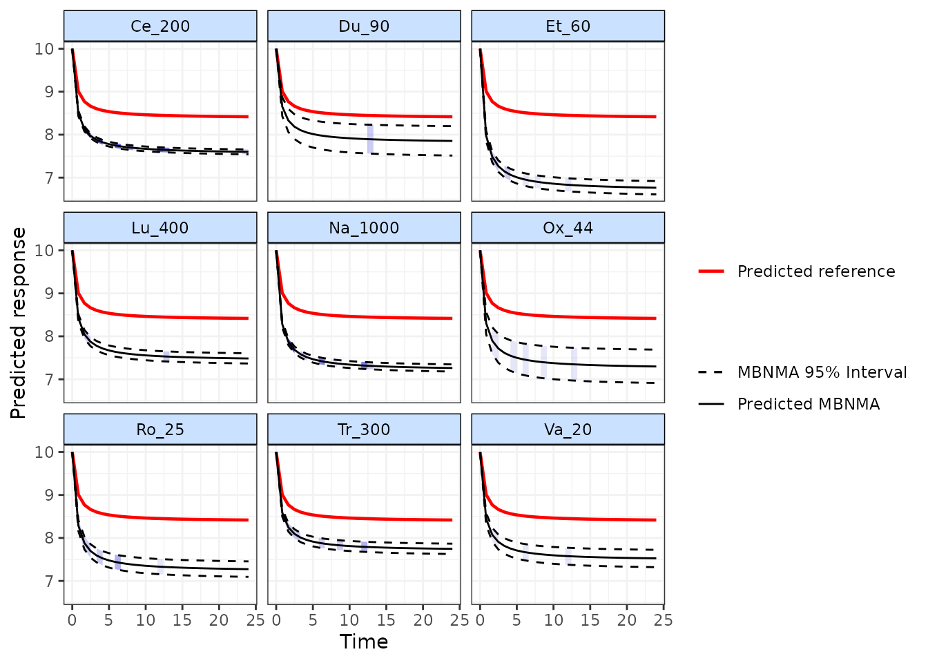
Predicted values can also be plotted using the plot() method on an object of class("mb.predict"). Within the default arguments, the median predicted network reference treatment effect is overlaid on the predictions for each treatment. Setting overlay.ref = FALSE prevents this and causes the network reference treatment effect to be plotted as a separate panel. Shaded counts of observations in the original dataset at each predicted time point can be plotted over the 95% CrI for each treatment by setting disp.obs = TRUE.

plot(pred, overlay.ref=TRUE, disp.obs=TRUE)

This can be used to identify any extrapolation/interpretation of the time-course that might be occurring for a particular treatment, and where predictions might therefore be problematic.

To illustrate a situation in which this could be very informative, we can look at predictions for a quadratic time-course function fitted to the Obesity dataset:

# Fit a quadratic time-course MBNMA to the Obesity dataset
network.obese <- mb.network(obesityBW_CFB, reference = "plac")

mbnma <- mb.run(network.obese,
                fun=tpoly(degree=2,
                          pool.1 = "rel", method.1="common",
                          pool.2="rel", method.2="common"))

# Define stochastic values centred at zero for network reference treatment
ref.params <- list(beta.1=~rnorm(n, 0, 0.05), beta.2=~rnorm(n, 0, 0.0001))

# Predict responses within the range of the data
pred.obese <- predict(mbnma, times=c(0:50), E0=100, treats = c(1,4,15),
                        ref.resp=ref.params)

# Plot predictions
plot(pred.obese, disp.obs = TRUE)

As you can see, within the limits of the observed data the predicted values appear reasonable. However, extrapolation beyond this for dexf_30MG leads to some rather strange results, suggesting an unrealistically huge increase in body weight after 50 weeks of treatment. On the other hand, the predicted response at 50 weeks follow-up in treatment 15 is within the limits of the observed data and so are likely to be more justifiable.

Plotting “lumped” NMA results

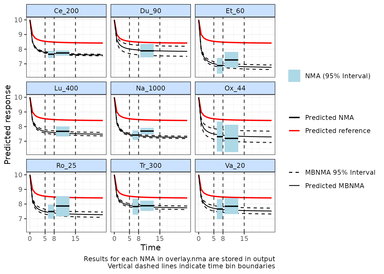
As a further addition to the plots of MBNMA predictions, it is possible to add predicted results from an NMA model or multiple “lumped” NMA models performed a different time “bins” (specified in overlay.nma), time periods within which we are assuming treatment effects are constant over time. This is similar to the output generated by binplot(). Either a "random" (the default) or "common" effects NMA can be specified, and model fit statistics are reported below the resulting plot.

This can be useful to assess if the MBNMA predictions are in agreement with predictions from lumped NMA models over a specific set of time-points, and can be a general indicator of the fit of the time-course model. However, it is important to note that the NMA model is not necessarily the more robust model, since it ignores potential differences in treatment effects that may arise from lumping time-points together. The wider the range specified in overlay.nma, the greater the effect of lumping and the stronger the assumption of similarity between studies.

The NMA predictions are plotted over the range specified in overlay.nma as a horizontal line representing the posterior median, with the 95%CrI shown by a shaded rectangle. The NMA predictions in theory represent those for any time-points within this range since they lump together data at all these time-points, though the width (x-axis) of the shaded rectangle represents the range of time-points for studies included in each time bin. Predictions for treatments that are disconnected from the network reference treatment at data points specified within overlay.nma cannot be estimated so are not included.

# Overlay predictions from lumped NMAs between 5-8 and between 8-15 weeks follow-up
plot(pred, overlay.nma=c(5,8,15), n.iter=20000)
#> Reference treatment in plots is Pl_0
#> Running overlay.nma for time=5 and time=8
#> Running overlay.nma for time=8 and time=15

Ranking

Predictions can also be ranked, allowing for ranking of predicted efficacy at a single time-point. We will illustrate this by ranking mean differences from the network reference treatment (i.e. by setting ref.resp=NULL and E0=0).

# Predict responses within the range of data
pred.obese <- predict(mbnma, times=c(0:50),
                      E0=0, ref.resp = NULL)
#> Priors required for: mu.1, mu.2
#> Success: Elements in prior match consistency time-course treatment effect parameters


# Rank predictions at 50 weeks follow-up
ranks <- rank(pred.obese, time=50)

summary(ranks)
#>              Length Class      Mode     
#> param             1 -none-     character
#> summary           8 data.frame list     
#> prob.matrix     676 -none-     numeric  
#> rank.matrix  117000 -none-     numeric  
#> cum.matrix      676 -none-     numeric  
#> lower_better      1 -none-     logical

plot(ranks)

The results indicate that dexf_60MG (Dexfenfluramine 60mg) is the highest ranked treatment.

Hugo Pedder