Forest plot for results from time-course MBNMA models

Generates a forest plot for time-course parameters of interest from results from time-course MBNMA models. Posterior densities are plotted above each result using ggdist:stat_:halfeye()

Usage

# S3 method for class 'mbnma'
plot(x, params = NULL, treat.labs = NULL, class.labs = NULL, ...)

Arguments

x

An S3 object of class "mbnma" generated by running a time-course MBNMA model

params

A character vector of time-course parameters to plot. Parameters must be given the same name as monitored nodes in mbnma and must vary by treatment or class. Can be set to NULL to include all available time-course parameters estimated by mbnma.

treat.labs

A character vector of treatment labels. If left as NULL (the default) then labels will be used as defined in the data.

class.labs

A character vector of class labels if mbnma was modelled using class effects If left as NULL (the default) then labels will be used as defined in the data.

...

Arguments to be sent to ggdist::stat_halfeye()

Value

A forest plot of class c("gg", "ggplot") that has separate panels for different time-course parameters

Examples

# \donttest{
# Create an mb.network object from a dataset
alognet <- mb.network(alog_pcfb)
#> Reference treatment is `placebo`
#> Studies reporting change from baseline automatically identified from the data

# Run an MBNMA model with an Emax time-course
emax <- mb.run(alognet,
  fun=temax(pool.emax="rel", method.emax="common",
    pool.et50="rel", method.et50="common"),
  intercept=FALSE)
#> 'et50' parameters must take positive values.
#>  Default half-normal prior restricts posterior to positive values.
#> Compiling model graph
#>    Resolving undeclared variables
#>    Allocating nodes
#> Graph information:
#>    Observed stochastic nodes: 233
#>    Unobserved stochastic nodes: 38
#>    Total graph size: 4166
#> 
#> Initializing model
#> 

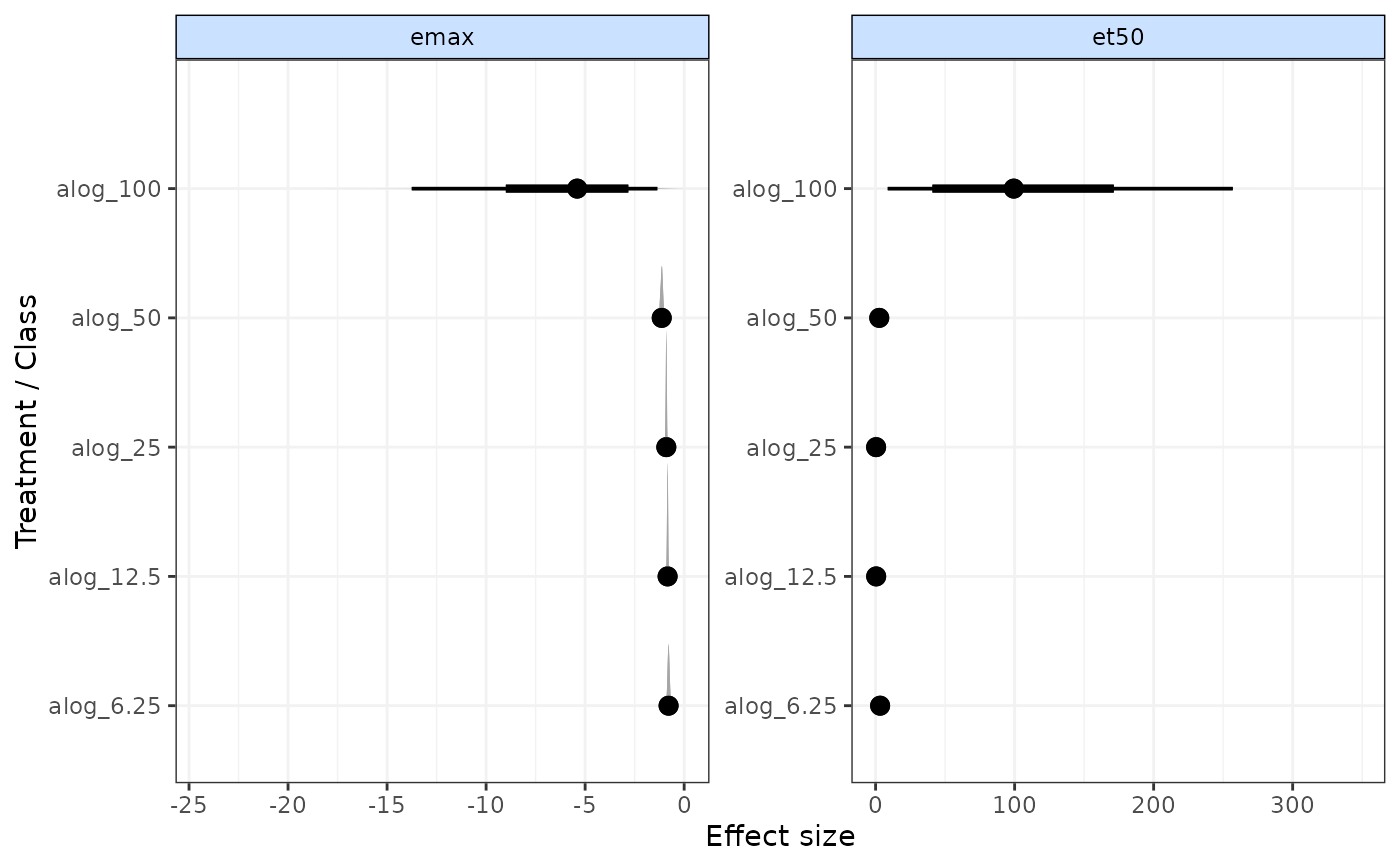
# Generate forest plot
plot(emax)


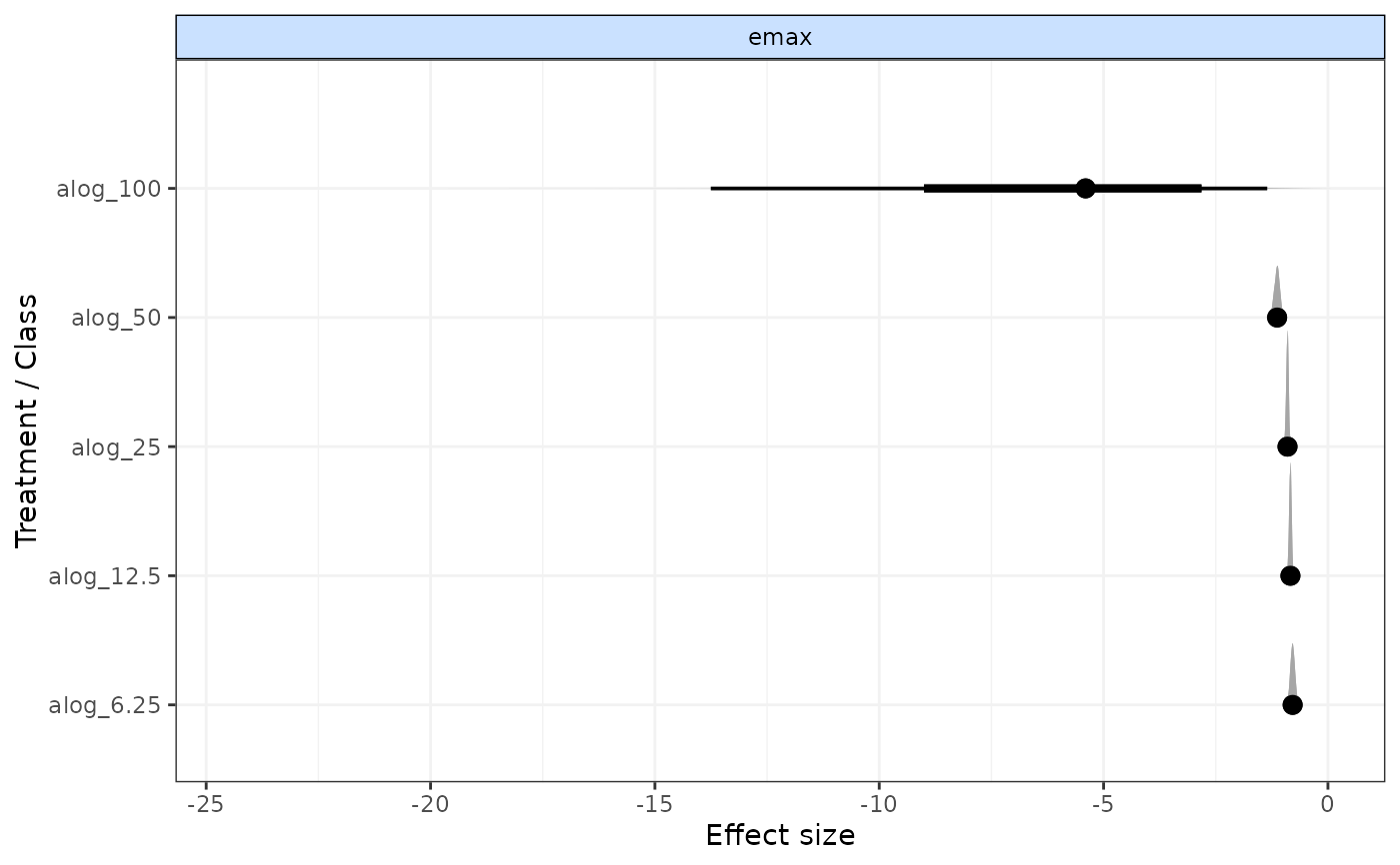
# Plot results for only one time-course parameter
plot(emax, params="emax")

# }