Perform node-splitting on a MBNMA time-course network

Within a MBNMA time-course network, split contributions into direct and indirect evidence and test for consistency between them. Closed loops of treatments in which it is possible to test for consistency are those in which direct and indirect evidence are available from independent sources van Valkenhoef van Valkenhoef et al. (2016) .

Usage

# S3 method for nodesplit
plot(x, plot.type = NULL, params = NULL, ...)

mb.nodesplit(
  network,
  comparisons = mb.nodesplit.comparisons(network),
  nodesplit.parameters = "all",
  fun = tpoly(degree = 1),
  times = NULL,
  lim = "cred",
  ...
)

Arguments

x: An object of class("nodesplit")
plot.type: A character string that can take the value of "forest" to plot only forest plots, "density" to plot only density plots, or left as NULL (the default) to plot both types of plot.
params: A character vector corresponding to a time-course parameter(s) for which to plot results. If left as NULL (the default), nodes-split results for all time-course parameters will be plotted.
...: Arguments to be sent to mb.run()
network: An object of class "mb.network".
comparisons: A data frame specifying the comparisons to be split (one row per comparison). The frame has two columns indicating each treatment for each comparison: t1 and t2.
nodesplit.parameters: A character vector of named time-course parameters on which to node-split (e.g. c("beta.1", "beta.2")). Can use "all" to split on all time-course parameters.
fun: An object of class "timefun" generated (see Details) using any of tloglin(), tpoly(), titp(), temax(), tfpoly(), tspline() or tuser()
times: A sequence of positive numbers indicating which time points to predict mean responses for (or at which to conduct a node-split if used with mb.nodesplit())
lim: Specifies calculation of either 95% credible intervals (lim="cred") or 95% prediction intervals (lim="pred").

Value

Plots the desired graph(s) and returns an object (or list of objects if plot.type=NULL) of class(c("gg", "ggplot")), which can be edited using ggplot commands.

A an object of class("mb.nodesplit") that is a list containing elements d.X.Y (treatment 1 = X, treatment 2 = Y). Each element (corresponding to each comparison) contains additional numbered elements corresponding to each parameter in the time-course function on which node splitting was performed. These elements then contain:

overlap matrix MCMC results for the difference between direct and indirect evidence
p.values Bayesian p-value for the test of consistency between direct and indirect evidence
quantiles
forest.plot
density.plot
direct MCMC results for the direct evidence
indirect MCMC results for the indirect evidence

Details

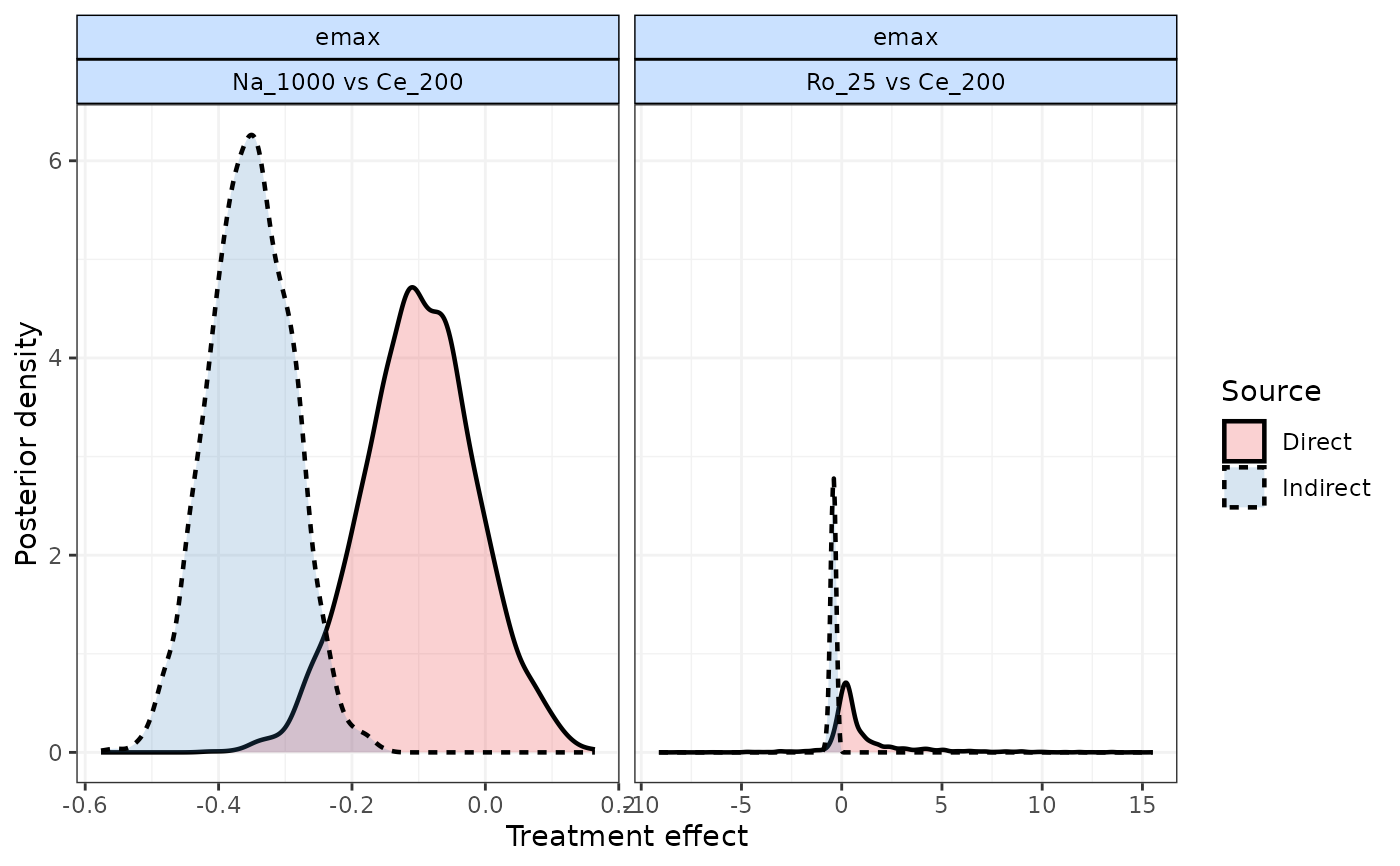
The S3 method plot() on an mb.nodesplit object generates either forest plots of posterior medians and 95\% credible intervals, or density plots of posterior densities for direct and indirect evidence.

Note that by specifying the times argument a user can perform a node-split of treatment effects at a specific time-point. This will give the treatment effect for both direct, indirect, and MBNMA estimates at this time point.

Functions

plot(nodesplit): Plot outputs from nodesplit models

References

van Valkenhoef G, Dias S, Ades AE, Welton NJ (2016). “Automated generation of node-splitting models for assessment of inconsistency in network meta-analysis.” Res Synth Methods, 7(1), 80-93. ISSN 1759-2887 (Electronic) 1759-2879 (Linking), doi:10.1002/jrsm.1167 , https://pubmed.ncbi.nlm.nih.gov/26461181/.

Examples

# \donttest{
# Create mb.network object
painnet <- mb.network(osteopain)
#> Reference treatment is `Pl_0`
#> Studies reporting change from baseline automatically identified from the data

# Identify comparisons informed by direct and indirect evidence
splits <- mb.nodesplit.comparisons(painnet)

# Fit a log-linear time-course MBNMA (takes a while to run)
result <- mb.nodesplit(painnet, comparisons=splits, nodesplit.parameters="all",
  fun=tloglin(pool.rate="rel", method.rate="common"),
  rho="dunif(0,1)", covar="varadj"
  )
#> running checks
#> Running NMA model
#> Compiling model graph
#>    Resolving undeclared variables
#>    Allocating nodes
#> Graph information:
#>    Observed stochastic nodes: 417
#>    Unobserved stochastic nodes: 89
#>    Total graph size: 7303
#> 
#> Initializing model
#> 
#> Comparison 1/2
#> Calculating nodesplit for: Ce_200 vs Ro_25
#> Treatment code: 3 vs 22
#> Compiling model graph
#>    Resolving undeclared variables
#>    Allocating nodes
#> Graph information:
#>    Observed stochastic nodes: 417
#>    Unobserved stochastic nodes: 467
#>    Total graph size: 7651
#> 
#> Initializing model
#> 
#> Direct complete
#> Reference treatment is `Pl_0`
#> Studies reporting change from baseline automatically identified from the data
#> Compiling model graph
#>    Resolving undeclared variables
#>    Allocating nodes
#> Graph information:
#>    Observed stochastic nodes: 414
#>    Unobserved stochastic nodes: 89
#>    Total graph size: 7251
#> 
#> Initializing model
#> 
#> Indirect complete
#> Comparison 2/2
#> Calculating nodesplit for: Ce_200 vs Na_1000
#> Treatment code: 3 vs 15
#> Compiling model graph
#>    Resolving undeclared variables
#>    Allocating nodes
#> Graph information:
#>    Observed stochastic nodes: 417
#>    Unobserved stochastic nodes: 467
#>    Total graph size: 7651
#> 
#> Initializing model
#> 
#> Direct complete
#> Reference treatment is `Pl_0`
#> Studies reporting change from baseline automatically identified from the data
#> Compiling model graph
#>    Resolving undeclared variables
#>    Allocating nodes
#> Graph information:
#>    Observed stochastic nodes: 408
#>    Unobserved stochastic nodes: 89
#>    Total graph size: 7149
#> 
#> Initializing model
#> 
#> Indirect complete

# Fit an emax time-course MBNMA with a node-split on emax parameters only
result <- mb.nodesplit(painnet, comparisons=splits, nodesplit.parameters="emax",
  fun=temax(pool.emax="rel", method.emax="common",
    pool.et50="rel", method.et50="common"))
#> 'et50' parameters must take positive values.
#>  Default half-normal prior restricts posterior to positive values.
#> running checks
#> Running NMA model
#> Compiling model graph
#>    Resolving undeclared variables
#>    Allocating nodes
#> Graph information:
#>    Observed stochastic nodes: 417
#>    Unobserved stochastic nodes: 146
#>    Total graph size: 8294
#> 
#> Initializing model
#> 
#> Comparison 1/2
#> Calculating nodesplit for: Ce_200 vs Ro_25
#> Treatment code: 3 vs 22
#> Compiling model graph
#>    Resolving undeclared variables
#>    Allocating nodes
#> Graph information:
#>    Observed stochastic nodes: 417
#>    Unobserved stochastic nodes: 524
#>    Total graph size: 8646
#> 
#> Initializing model
#> 
#> Direct complete
#> Reference treatment is `Pl_0`
#> Studies reporting change from baseline automatically identified from the data
#> Compiling model graph
#>    Resolving undeclared variables
#>    Allocating nodes
#> Graph information:
#>    Observed stochastic nodes: 414
#>    Unobserved stochastic nodes: 146
#>    Total graph size: 8237
#> 
#> Initializing model
#> 
#> Indirect complete
#> Comparison 2/2
#> Calculating nodesplit for: Ce_200 vs Na_1000
#> Treatment code: 3 vs 15
#> Compiling model graph
#>    Resolving undeclared variables
#>    Allocating nodes
#> Graph information:
#>    Observed stochastic nodes: 417
#>    Unobserved stochastic nodes: 524
#>    Total graph size: 8646
#> 
#> Initializing model
#> 
#> Direct complete
#> Reference treatment is `Pl_0`
#> Studies reporting change from baseline automatically identified from the data
#> Compiling model graph
#>    Resolving undeclared variables
#>    Allocating nodes
#> Graph information:
#>    Observed stochastic nodes: 408
#>    Unobserved stochastic nodes: 146
#>    Total graph size: 8118
#> 
#> Initializing model
#> 
#> Indirect complete

# Inspect results
print(result)
#> ========================================
#> Node-splitting analysis of inconsistency
#> ========================================
#> 
#> emax
#> 
#> |Comparison        | p-value| Median|   2.5%|  97.5%|
#> |:-----------------|-------:|------:|------:|------:|
#> |Ro_25 vs Ce_200   |   0.480|       |       |       |
#> |-> direct         |        | -0.458| -2.452|  5.710|
#> |-> indirect       |        | -0.413| -0.720| -0.165|
#> |                  |        |       |       |       |
#> |Na_1000 vs Ce_200 |   0.461|       |       |       |
#> |-> direct         |        | -0.470| -1.050|  0.017|
#> |-> indirect       |        | -0.437| -0.571| -0.305|
#> |                  |        |       |       |       |
summary(result)
#>          Comparison Time.Param Evidence Median   2.5%  97.5% p.value
#> 1   Ro_25 vs Ce_200       emax   Direct -0.458 -2.452  5.710   0.480
#> 2   Ro_25 vs Ce_200       emax Indirect -0.413 -0.720 -0.165   0.480
#> 3 Na_1000 vs Ce_200       emax   Direct -0.470 -1.050  0.017   0.461
#> 4 Na_1000 vs Ce_200       emax Indirect -0.437 -0.571 -0.305   0.461

# Plot results
plot(result)


# }