Run an NMA model
nma.run.RdUsed for calculating treatment-level NMA results, either when comparing MBNMA models to models that
make no assumptions regarding dose-response , or to estimate split results for overlay.split.
Results can also be compared between consistency (UME=FALSE) and inconsistency
(UME=TRUE) models to test the validity of the consistency assumption at the treatment-level.
# S3 method for class 'nma'
plot(x, bydose = TRUE, scales = "free_x", ...)

nma.run(
  network,
  method = "common",
  likelihood = NULL,
  link = NULL,
  priors = NULL,
  sdscale = FALSE,
  warn.rhat = TRUE,
  n.iter = 20000,
  drop.discon = TRUE,
  UME = FALSE,
  pD = TRUE,
  parameters.to.save = NULL,
  ...
)
Arguments
- x
An object of
class("nma")- bydose
A boolean object indicating whether to plot responses with dose on the x-axis (
TRUE) to be able to examine potential dose-response shapes, or to plot a conventional forest plot with all treatments on the same plot (FALSE)- scales
Should scales be fixed (
"fixed", the default), free ("free"), or free in one dimension ("free_x","free_y")?- ...
Arguments to be sent to
ggplot2::ggplot()- network
An object of class
mbnma.network.- method
Indicates the type of split (treatment-level) NMA to perform when
overlay.split=TRUE. Can take either"common"or"random".- likelihood
A string indicating the likelihood to use in the model. Can take either
"binomial","normal"or"poisson". If left asNULLthe likelihood will be inferred from the data.- link
A string indicating the link function to use in the model. Can take any link function defined within JAGS (e.g.
"logit","log","probit","cloglog"), be assigned the value"identity"for an identity link function, or be assigned the value"smd"for modelling Standardised Mean Differences using an identity link function. If left asNULLthe link function will be automatically assigned based on the likelihood.- priors
A named list of parameter values (without indices) and replacement prior distribution values given as strings using distributions as specified in JAGS syntax (see Plummer (2017) ). Note that normal distributions in JAGS are specified as $$N(\mu, prec)$$, where $$prec = 1 / {\sigma^2}$$.
- sdscale
Logical object to indicate whether to write a model that specifies a reference SD for standardising when modelling using Standardised Mean Differences. Specifying
sdscale=TRUEwill therefore only modify the model if link function is set to SMD (link="smd").- warn.rhat
A boolean object to indicate whether to return a warning if Rhat values for any monitored parameter are >1.02 (suggestive of non-convergence).
- n.iter
number of total iterations per chain (including burn in; default: 20000)
- drop.discon
A boolean object that indicates whether or not to drop disconnected studies from the network.
- UME
A boolean object to indicate whether to fit an Unrelated Mean Effects model that does not assume consistency and so can be used to test if the consistency assumption is valid.
- pD
logical; if
TRUE(the default) then adds the computation of pD, using the method of (Plummer 2008) . IfFALSEthen uses the approximation ofpD=var(deviance) / 2(often referred to as pV).- parameters.to.save
A character vector containing names of parameters to monitor in JAGS
Functions
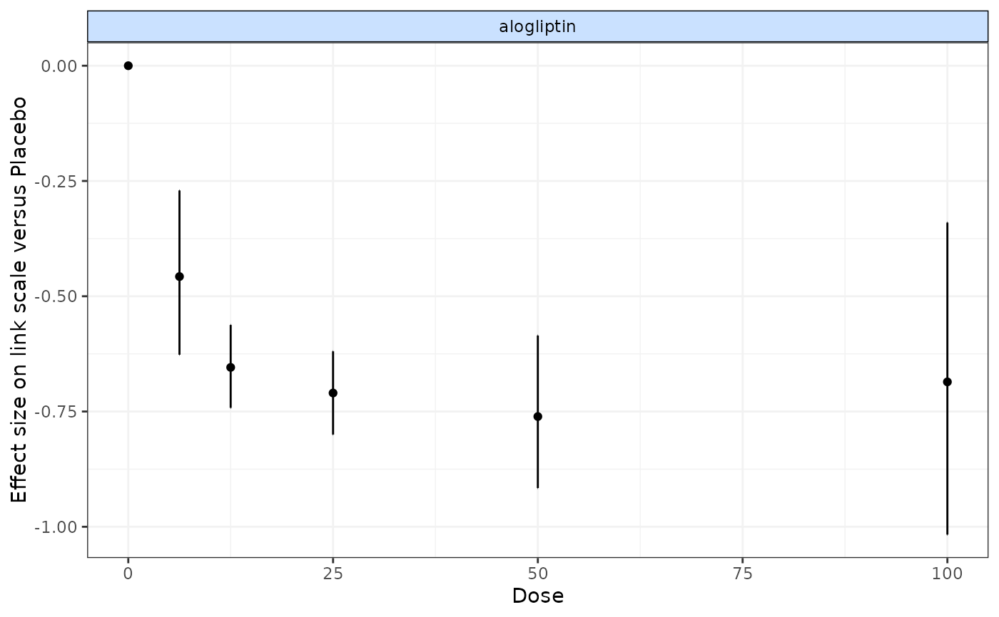
plot(nma): Plot outputs from treatment-level NMA modelsResults can be plotted either as a single forest plot, or facetted by agent and plotted with increasing dose in order to identify potential dose-response relationships. If Placebo (or any agents with dose=0) is included in the network then this will be used as the reference treatment, but if it is not then results will be plotted versus the network reference used in the NMA object (
x).
Examples
# \donttest{
# Run random effects NMA on the alogliptin dataset
alognet <- mbnma.network(alog_pcfb)
#> Values for `agent` with dose = 0 have been recoded to `Placebo`
#> agent is being recoded to enforce sequential numbering
nma <- nma.run(alognet, method="random")
#> Compiling model graph
#>    Resolving undeclared variables
#>    Allocating nodes
#> Graph information:
#>    Observed stochastic nodes: 46
#>    Unobserved stochastic nodes: 52
#>    Total graph size: 641
#>
#> Initializing model
#>
print(nma)
#> $jagsresult
#> Inference for Bugs model at "/tmp/Rtmp8BRYQO/file1aad698a5a25", fit using jags,
#>  3 chains, each with 20000 iterations (first 10000 discarded), n.thin = 10
#>  n.sims = 3000 iterations saved. Running time = 1.282 secs
#>            mu.vect sd.vect     2.5%      25%      50%      75%    97.5%  Rhat
#> d[1]         0.000   0.000    0.000    0.000    0.000    0.000    0.000 1.000
#> d[2]        -0.454   0.089   -0.628   -0.516   -0.454   -0.396   -0.279 1.002
#> d[3]        -0.653   0.045   -0.742   -0.684   -0.652   -0.623   -0.562 1.002
#> d[4]        -0.710   0.045   -0.798   -0.740   -0.710   -0.681   -0.619 1.001
#> d[5]        -0.761   0.085   -0.924   -0.816   -0.763   -0.705   -0.591 1.001
#> d[6]        -0.683   0.174   -1.015   -0.801   -0.682   -0.569   -0.334 1.001
#> sd           0.123   0.028    0.075    0.105    0.121    0.141    0.183 1.001
#> totresdev   47.191   9.933   30.365   40.036   46.254   53.558   68.162 1.001
#> deviance  -124.123   9.933 -140.949 -131.278 -125.060 -117.756 -103.152 1.001
#>           n.eff
#> d[1]          1
#> d[2]       1900
#> d[3]       1400
#> d[4]       3000
#> d[5]       3000
#> d[6]       3000
#> sd         2900
#> totresdev  3000
#> deviance   3000
#>
#> For each parameter, n.eff is a crude measure of effective sample size,
#> and Rhat is the potential scale reduction factor (at convergence, Rhat=1).
#>
#> DIC info (using the rule: pV = var(deviance)/2)
#> pV = 49.4 and DIC = -74.8
#> DIC is an estimate of expected predictive error (lower deviance is better).
#>
#> $trt.labs
#> [1] "Placebo_0"       "alogliptin_6.25" "alogliptin_12.5" "alogliptin_25"
#> [5] "alogliptin_50"   "alogliptin_100"
#>
#> $UME
#> [1] FALSE
#>
#> attr(,"class")
#> [1] "nma"
plot(nma)


# Run common effects NMA keeping treatments that are disconnected in the NMA
goutnet <- mbnma.network(gout)
#> Values for `agent` with dose = 0 have been recoded to `Placebo`
#> agent is being recoded to enforce sequential numbering
nma <- nma.run(goutnet, method="common", drop.discon=FALSE)
#> Compiling model graph
#>    Resolving undeclared variables
#>    Allocating nodes
#> Graph information:
#>    Observed stochastic nodes: 27
#>    Unobserved stochastic nodes: 28
#>    Total graph size: 296
#>
#> Initializing model
#>

# Run an Unrelated Mean Effects (UME) inconsistency model on triptans dataset
tripnet <- mbnma.network(triptans)
#> Values for `agent` with dose = 0 have been recoded to `Placebo`
#> agent is being recoded to enforce sequential numbering
ume <- nma.run(tripnet, method="random", UME=TRUE)
#> Compiling model graph
#>    Resolving undeclared variables
#>    Allocating nodes
#> Graph information:
#>    Observed stochastic nodes: 182
#>    Unobserved stochastic nodes: 436
#>    Total graph size: 4072
#>
#> Initializing model
#>
# }
# Run common effects NMA keeping treatments that are disconnected in the NMA
goutnet <- mbnma.network(gout)
#> Values for `agent` with dose = 0 have been recoded to `Placebo`
#> agent is being recoded to enforce sequential numbering
nma <- nma.run(goutnet, method="common", drop.discon=FALSE)
#> Compiling model graph
#> Resolving undeclared variables
#> Allocating nodes
#> Graph information:
#> Observed stochastic nodes: 27
#> Unobserved stochastic nodes: 28
#> Total graph size: 296
#>
#> Initializing model
#>
# Run an Unrelated Mean Effects (UME) inconsistency model on triptans dataset
tripnet <- mbnma.network(triptans)
#> Values for `agent` with dose = 0 have been recoded to `Placebo`
#> agent is being recoded to enforce sequential numbering
ume <- nma.run(tripnet, method="random", UME=TRUE)
#> Compiling model graph
#> Resolving undeclared variables
#> Allocating nodes
#> Graph information:
#> Observed stochastic nodes: 182
#> Unobserved stochastic nodes: 436
#> Total graph size: 4072
#>
#> Initializing model
#>
# }